Code used for this post.

Background

This post is about an analysis I did for a colleague involving some MiSeq data during my PhD. The problem was I couldn’t make sense of the data and needed to rule out a source of error that might have occurred during the sample generation process. The short of it was I used Monte Carlo simulation of that sample generation process and found that that potential source of error was not a concern. Unfortunately, (for additional reasons not discussed here) I had to conclude that the sample labels somehow got mixed up and were unusable. But the Monte Carlo simulations were instructive and I wanted to share what I did.

My colleague had collected ~90ish genomic DNA samples from cancer patient. There are at least two samples from each patient (one from healthy tissue and at least one from the tumor). He then amplified the genomic DNA using the REPLI-g kit (designed for low input amounts) [1], then amplified the exons of his gene of interest with the TruSeq kit [2], and sequenced with a MiSeq machine. The atypical aspect of his samples was the very low DNA amount in some samples.

After sequencing, my job was to identify the somatic mutations, but for a quality check on the data I also identified any germline mutations. Usually, germline mutations present in the healthy tissue should also be present in the tumor (though loss of heterozygosity and copy number aberrations can occur). But what I found was not at all consistent with that assumption. Some normal and tumor samples from the same patient all had a germline mutation, but most didn’t. So one possibility was erroneous mutations were being introduced during the sample generation process. It is well known that PCR can (at very low probability) introduce mutations (Figure 1). Moreover, I knew that some of these samples started from tiny amounts of genomic DNA before undergoing the two PCR amplifications (the REPLI-g and TruSeq kits). When you start with smaller and smaller amounts of DNA, mutations introduced during PCR amplification can be present at higher frequencies in the end product [3,4].

Figure 1: A PCR might have anywhere between 10 and 30 cycles, where in each cycle the DNA fragments are duplicated. The proteins that duplicate the DNA are not perfect and can introduce mutations that can propagate.

Methods

I used Monte Carlo stochastic simulations to estimate the maximum frequency which I can expect PCR errors to appear in the final sequenced sample. The general outline of my modeling approach is shown in Figure 2. The two PCR steps are modeled using a multi-type branching process, and there is an additional step in between them that uses binomial sampling to simulate taking a small sample of the first PCR product. In addition to those three basic steps, there are some additional parameters that I varied during my Monte Carlo runs (Table 1). The range in parameter values are based on the details of the sample preparation kits and on information provided to me by my colleague.

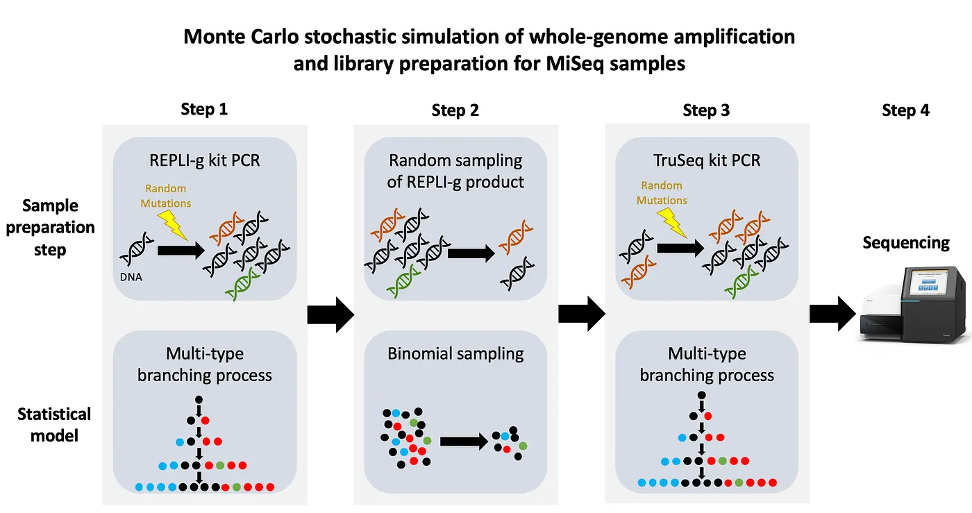
Figure 2: The three step process from starting with the genomic DNA sample from the patient and ending in the sequenced data. The top row shows the step in sample preparation, while the bottom row shows how it was modeled mathematically. There are of course more steps taken by the biologist handling the samples, but the important parts are shown here.

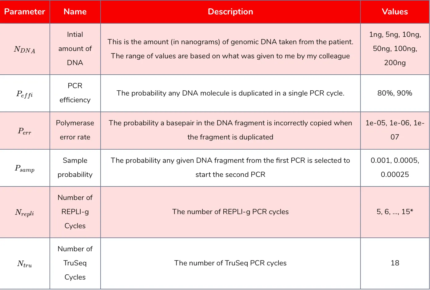
Table 1: parameters varied in the Monte Carlo simulation. *Fewer REPLI-g cycles were used for larger starting amounts of DNA due to computational limitations.

The full steps for the Monte Carlo simulation are as follows (repeated 100 times for each parameter combination):

Step 1: Generate DNA population: Generate a population of DNA fragments using 1’s and 0’s to represent DNA (to simplify things). The size of a fragment is equal to the size of the sequenced area in the MiSeq data (3,172 basepairs). How many DNA fragments correspond to a given nanogram amount of DNA (N_dna) is based on the literature.

Step 2: REPLI-g PCR: Simulate N_repli PCR cycles. Each cycle a DNA fragment has a probability P_effi of being duplicated. Each basepair in the DNA fragment has a probability P_err of being copied wrong.

Step 3: Binomial sampling: Sample each DNA fragment from Step 2 with probability P_samp.

Step 4: TruSeq PCR: Simulate N_tru PCR cycles. Each cycle a DNA fragment has a probability P_effi of being duplicated. Each basepair the DNA fragment has a probability P_err of being copied wrong.

Results

I performed 100 simulations for each parameter combination. At the end of each simulation I identified the mutation (resulting from PCR error) with maximum allele frequency, which I will call maximum variant allele frequency (MVAF). Figures 3, 4, and 5 plot the MVAF values against the various parameter settings. The resulting trends generally make sense. All three figures show that with smaller starting amounts of DNA you can get values of MVAF. Higher polymerase error rates, less PCR efficiency, and taking a smaller sample between the PCR steps can also all result in higher MVAF values. However, the important finding is that the MVAF values never get much higher than 2%. And keep in mind that MVAF only records the PCR error with the highest frequency in the simulation; there can be tens to hundreds of other PCR errors that occurred in the simulation. Hence, these results indicate that the mutations that I am observing in my dataset are unlikely to be the result of PCR errors.

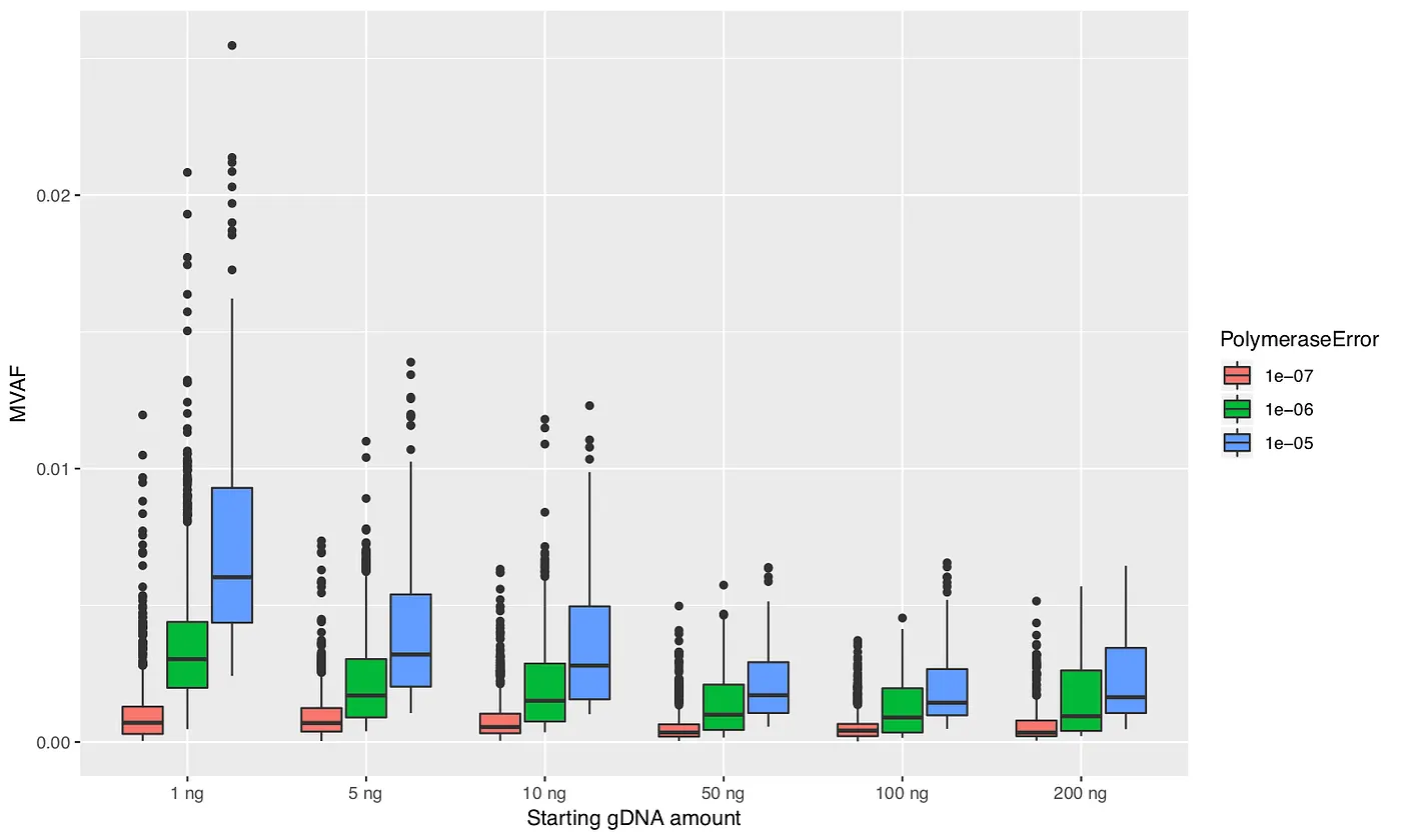
Figure 3: Maximum variant allele frequency (MVAF) values for various amounts of starting DNA and polymerase error rates.

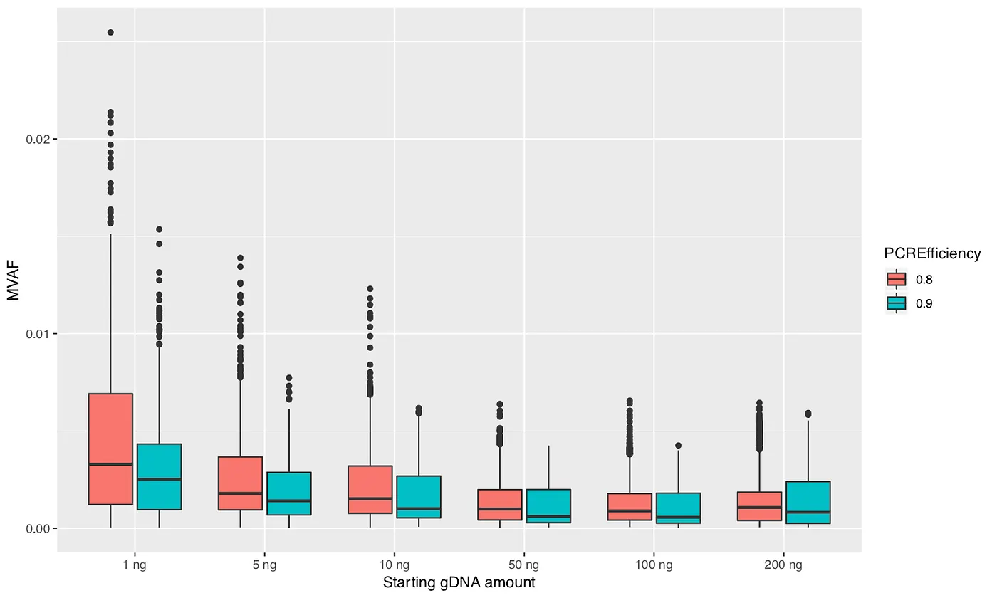
Figure 4: Maximum variant allele frequency (MVAF) values for various amounts of starting DNA and polymerase error rates.

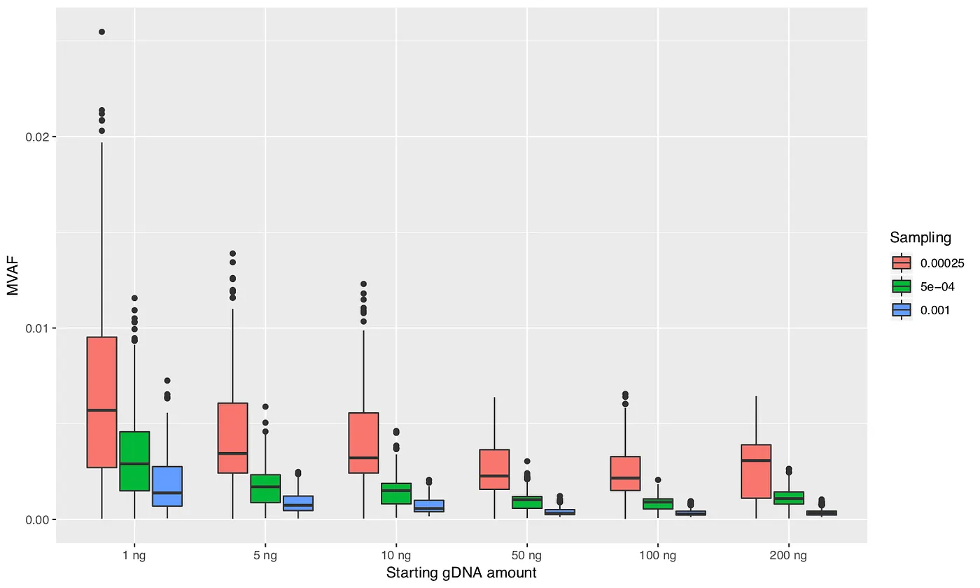
Figure 5: Maximum variant allele frequency (MVAF) values for various amounts of starting DNA and polymerase error rates.

Conclusions

I concluded from this study that PCR errors were not a cause for concern in my dataset. Even with the smallest amount of starting DNA, highest polymerase error rates, and smallest sampling rate in between the two PCRs, the final frequency of PCR errors only got as high as a few percent. Whereas I was looking to see if the frequencies could go 40% or higher becase germline mutations are expected to be around either 50% or 100%. So I could only conclude that the germline mutation mismatch I found in samples from the same patient were caused by sample label mixup.

But I should note that there were some simplifying assumptions that I made which could affect the results, including:

• I modeled DNA using just 0’s and 1’s instead of the four letter alphabet (A, T, C, G). I don’t think this would make a big difference in my findings though.
• I limited the number of PCR cycles simulated for computational reasons. Doing more cycles could result in PCR errors that achieve higher frequency.

References

1. REPLI-g Mini Kit
2. TruSeq DNA Library Prep Kits
3. Kebschull JM, Zador AM. Sources of PCR-induced distortions in high-throughput sequencing data sets. Nucleic Acids Research. 2015 Dec 2;43(21):e143–15.
4. Best K, Oakes T, Heather JM, Shawe-Taylor J, Chain B. Computational analysis of stochastic heterogeneity in PCR amplification efficiency revealed by single molecule barcoding. Sci Rep. Nature Publishing Group; 2016 Mar 4;:1–13.