Code for this post.

Background

One of my papers involved sequencing the tumors of a mouse model of triple-negative breast cancer (TNBC) [1]. We sequenced the tumors using RNA-seq data. If you’re not familiar with these technology, RNA-seq sequences the RNA transcripts to tell you what parts of the genome are expressed [2].

Our mouse model was genetically engineered to develop TNBC by deleting the Trp53 gene. We also deleted the Brca1 gene in 50% of the mice as well since we wanted to study how that gene influences tumor development (see Table 1 for our samples). Hence, the mouse tumors had one of two genotypes: Trp53-deleted/Brca1-wildtype or Trp53-deleted/Brca1-deleted (wildtype just means the gene was not deleted or altered). Because genetic engineering is not always perfect and sample mix-ups can happen, we needed to validate the genotype for each mouse. We can do this by looking at the sequencing data. If a gene is deleted in a sample we should not see any evidence for it in the RNA-seq data (Figure 1).

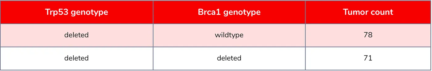
Table 1: Number of samples per genotype.

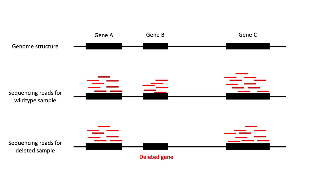
Figure 1: Sequenced reads (in red) from WES are sampled as short fragments from the genome. (Top row) Shows an example genome with three genes. (Middle row) Shows sequencing reads from a sample with wildtype genotype. Reads are sampled from each gene. (Bottom row) Shows a sample with gene B deleted. No reads are samples from gene B.

I detail here the process I took to validate the genotypes of the mouse tumors in my paper [1]. Some of the tumors could not be genotyped using conventional molecular biology methods, so when we sequenced the tumor we did not know its genotype. Moreover, we also suspected that some samples might have been genotyped incorrectly based on our observations from PCA.

Data preparation

RNA-seq data provides insight into how the thousands of genes of a sample are being expressed (the transcriptome), and is strongly influenced by the presence of absence of genes. Hence, we hypothesized that we will see a global effect on the transcriptome when comparing Brca1 genotypes. Figure 2 (left) shows a PCA on the expression profile of all tumors (14,137 genes and 149 samples). The Brca1 genotype has a huge impact on the transcriptome of a sample and seems to explain most of the variance. The figure also shows that there are some outlier or potentially mislabelled samples. I chose to remove those outlier samples prior to training my model (Figure 2, right).

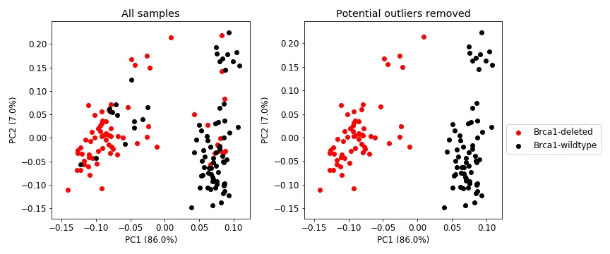
Figure 2: PCA plot showing PC1 and PC2, and percent variance explained in parentheses. PCA was performed on the RNA-seq data (14,137 genes and 149 samples). Brca1 has a huge impact on a sample’s transcriptome and explains most of the data’s variance. The figure also shows some potentially mislabelled or outlier samples.

One additional complexity about this data needs to be introduced. In Brca1-deleted samples, the whole Brca1 gene is not deleted, but only a portion of it (the functionally important part of it). The mouse Brca1 gene has 23 exons, and only exons 4 to 12 are deleted in the Brca1-deleted samples. So when we look at the number of reads mapping to each exon in the RNA-seq, we should ideally see no reads mapping to exons 4 to 12. However, as shown in Figures 3 and 4, we will not always see such a clean case due to various reason. Figures 3 shows that there is definitely some discriminatory power in exons 4 to 12, but there are still some Brca1-deleted samples with read counts similar to Brca1-wildtype. Figure 4 shows a PCA plot using the data in Figure 3 where the samples were treated as variables. Figures 3 and 4 both show a general separation of samples by Brca1 genotype, but it is not perfect. Potential reasons for this include:

1. The sample was mislabelled
2. The process to generate Brca1-deleted genotype was not effective
3. The sample might be contaminated with tissue that is Brca1-wildtype. This can happen because the Brca1 gene was not intended to be deleted in the whole mouse, but only in the tissue the tumor arose from.

The challenge was then to build a classifier using the data in Figure 3 so I could correct any mislabelled samples and predict the Brca1 genotype for those we lacked the information for.

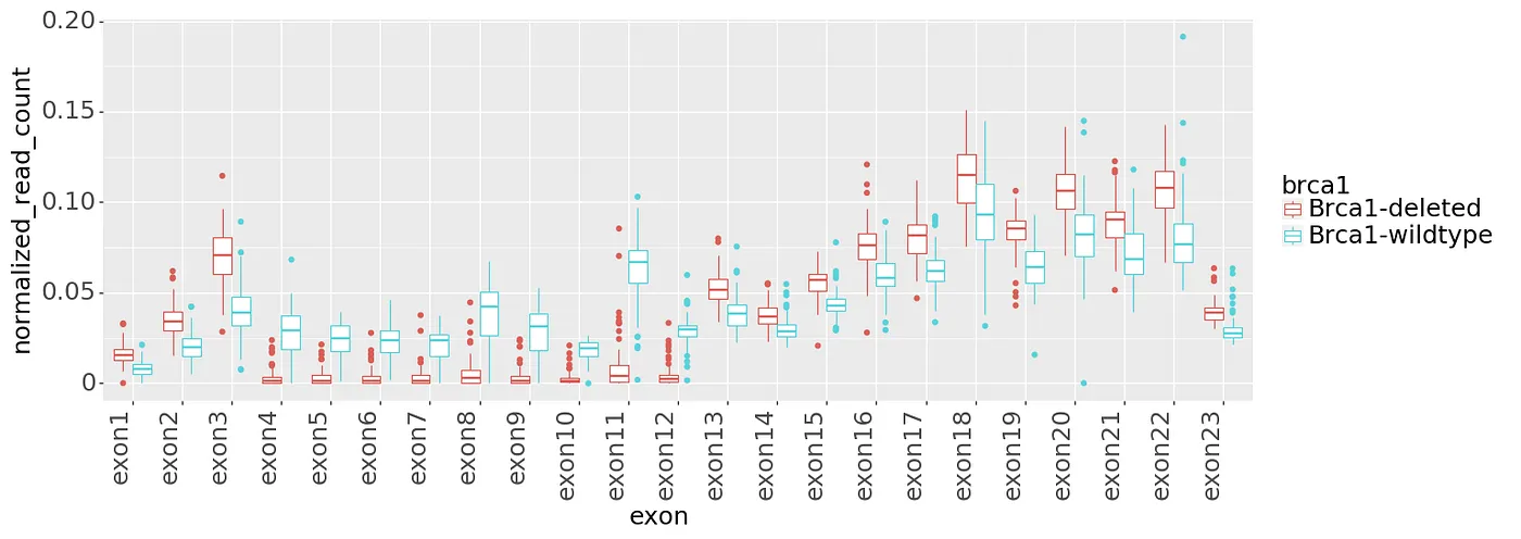
Figure 3: Normalized read counts per Brca1 exon.

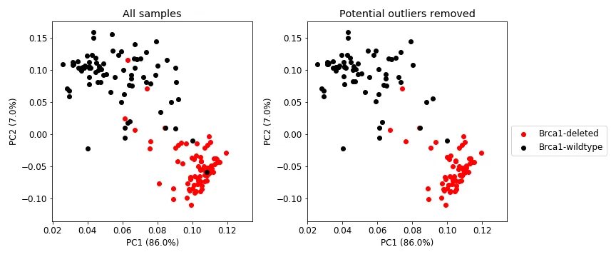
Figure 4: PCA on the exon expression data using the samples as variables. Left: shows all samples. Right: shows only those samples that were not removed in Figure 2, right.

Modelling

There are 23 exons, so there are 23 variables in this dataset. Initially I thought just exons 4–12 are needed to build a classifier, but Figure 3 indicates the other exons might be useful too. However, one issue with the date (whether just exons 4–12 or all of them), is the abundant collinearity among the variables (Figures 5 and 6). PCA shows that the first PC explains over 60% of the variance, and ~90% in the first 5 PCs. The scatter plot (Figure 6) shows how correlation between exons increases between neighboring ones, and that exons 4–12 are much higher correlation among themselves compared to the rest.

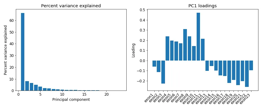
Figure 5: PCA on the normalized read count per Brca1 exon from Figure 3. Left figure shows the percent variance explained by each principal component (PC). Right figure shows the per-exon loadings for the first PC.

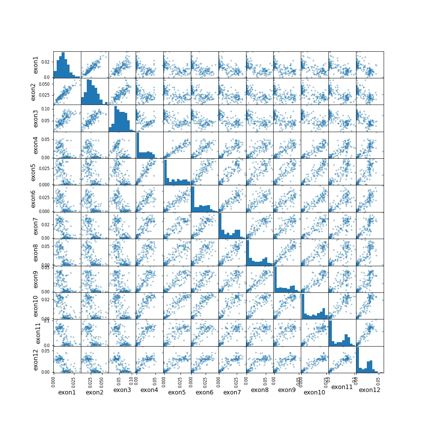
Figure 6: Scatter plots for exons 1–13. Exons closer together seem to have higher correlation, and exons 4–12 have particularly high correlation among themselves.

The collinearity in this dataset indicated that I might want to use PCA to reduce dimensionality. I did try this (results are in the Jupyter notebook), but it did not do better than other models that used all exons as variables. The models I tried that use all 23 exons are:

• Decision tree
• LDA
• LDA with shrinkage -Linear SVC
• Nonlinear SVC
• Plain logistic regression
• Logistic regression with l1 shrinkage
• Logistic regression with l2 shrinkage

The results from cross-validation and parameter optimization are in Figure 7 and Table 2. They all perform pretty well, though LDA, plain logistic regression, and logistic regression with l1 did tiny bit worse. Rerunning cross validation on all the models can lead to slightly different results, so I just went with logistic regression (with l2 regularization) for ease of interoperability. Figure 8 shows the per exon coefficients from the model.

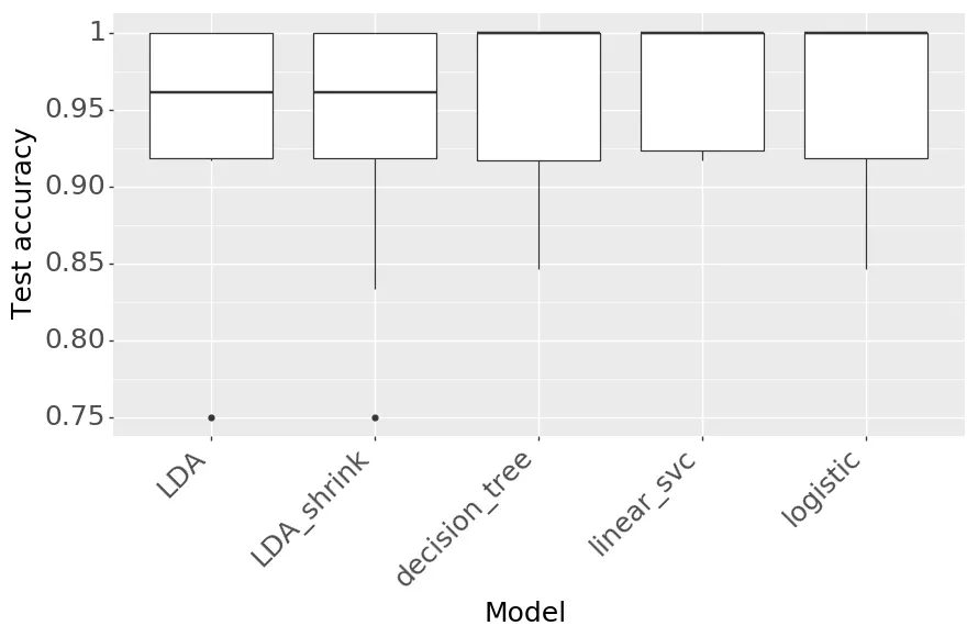
Figure 7: Comparison of model accuracies (10-fold CV)

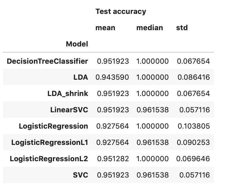
Table 2: Comparison of model accuracies (10-fold CV)

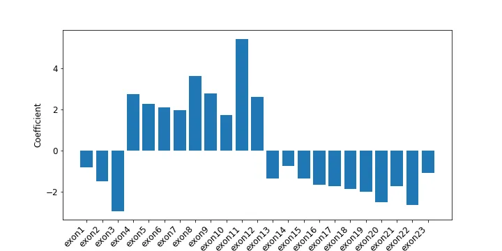
Figure 8: Per-exon coefficients from logistic regression with l2.

Model application

I applied the logistic regression (with l2) to see which samples are mislabelled. Figures 9, 10 and 11 all show the same genotype prediction but highlight different sample subsets. The plots on the left show the PCA on the transcriptional profile (as was shown in Figure 2). Similarly the plots on the right show the PCA on the exon expression profile (as was shown in Figure 4).

Even after predicting each sample’s genotype, the transcriptional profiles still does not clearly differential Brca1 genotype (Figure 9, left). However, a sample’s exon expression profile does (Figure 9, right). Regardless of where the sample is on the transcriptome PCA plot (Figure 10, left), its newly assigned Brca1 genotype relatively makes sense when you look at where it lies in the exon expression PCA plot (Figure 10, right); that is, samples cluster pretty well by Brca1 genotype in. Finally, the samples that were removed as outliers for the most part did not change genotype (Figure 11). Indicating that their originally assigned genotype is correct.

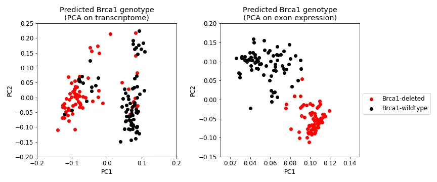
Figure 9: Genotype predictions for all samples. Shows the same data as in Figure 4, except the Brca1 genotype is predicted. Left: First two PCs from transcriptional data. Right: First two PCs from exon expression data.

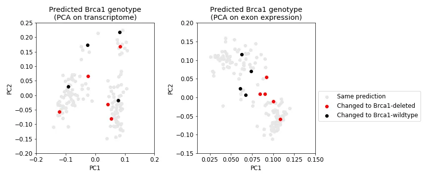
Figure 10: Samples that change genotype. Shows the same data as in Figure 9 but highlights those samples whose predicted genotype is different than what was originally given.

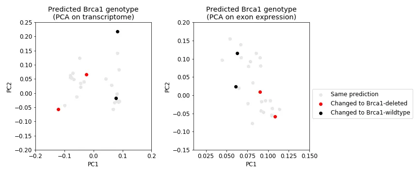
Figure 11: Outlier samples that change genotype. Shows the same data as in Figure 10 but only shows those samples that were removed as outliers in Figure 2.

Conclusions

Biology (and cancer biology) is complex and phenotype does not always correlate with genotype. Although Brca1 genotype status dominates each sample’s transcriptional profile, it isn’t always the case. Samples that have Brca1-deleted genotype sometimes look (phenotypically) like Brca1-wildtype and vice versa. There are a myriad of potential ways cancer can either regain or lose function of gene through things likes mutation, copy number aberrations, signaling pathways, etc… So it should not be too much of a surprise how a sample’s transcriptional profile does not perfectly reflect its Brca1 genotype.

I used the expression profile of the Brca1 exons to build a classifier for Brca1 genotype. Exploratory plots of the data indicated pretty obvious discriminatory power, although there is quite a bit of collinearity. Attempts to reduce collinearity with PCA and then build a classifier did not outperform models with regularization. I ended up choosing a regularized logistic regression model for its ease of interoperability.

I identified many potentially mislabelled samples by looking at a PCA plot of transcriptional profiles, which uses the expression profile of ~14,000 genes on each sample. After removing those potentially mislabelled samples I built the classifier. Dispute achieving > 95% accuracy, most of those samples were predicted to have the same genotype they were originally assigned. Indicating that those samples found some way to look phenotypically like their opposite Brca1 genotype.

References

1. Liu H, Murphy CJ, Karreth FA, Emdal KB, Yang K, White FM, et al. Identifying and Targeting Sporadic Oncogenic Genetic Aberrations in Mouse Models of Triple-Negative Breast Cancer. Cancer Discovery. 2017 Dec 4;8(3):354–69.
2. Wang Z, Gerstein M, Snyder M. RNA-Seq: a revolutionary tool for transcriptomics. Nature Publishing Group. 2009 Jan;10(1):57–63.