
Background
I encountered heteroskedasticity while calling copy number abberations (CNA) from whole-exome sequencing (WES) data in tumors. CNAs happen when parts of or whole chromosomes gain or lose one or more copies (we all have two copies of each chromosomes). CNAs frequently occur in cancer, so detecting them is important [1]. Calling CNAs these days is often done using WES or whole-genome sequencing. Figure 1 shows example CNA calls for one tumor sample.
DNA fragments would ideally be uniformly sampled from throughout the genome, but Illumina sequencing machines (for example) tend to have a bias with very high or low GC content. GC content is the number G and C basepairs in the sequenced read. Other biases in sampling the genome may also occur. However, this is usually dealt with by sequencing a paired normal tissue sample from the same patient. The normal control sample then has those same biases, so when you compute a log ratio of the tumor over normal control, the biases cancel out. However, the reason why I am writing this post is I had the unfortunate experience with having data where those biases did not cancel out [2]. Figure 2 shows the issue that caused it. It plots the log2(tumor/control) against the GC content. Normally this would appear flat, but there is clear heteroskedasticity with respect to GC content, which was undesirable. To more clearly show the heteroskedasticity, Figure 3 shows the variance estimate in windows of 0.005 GC content.
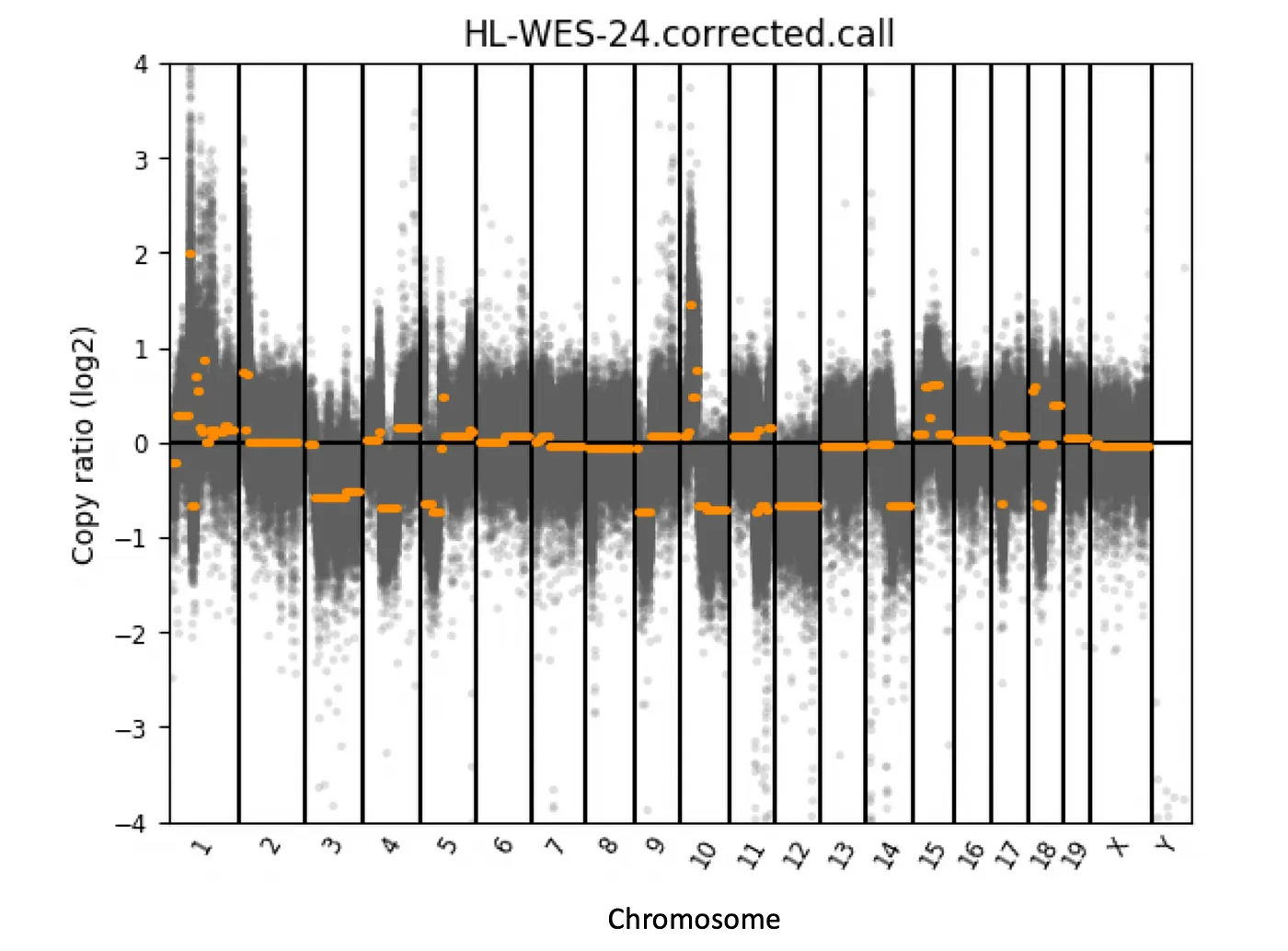
Figure 1: CNA calls from a example tumor. The copy ratio (log2) is the ratio of read coverage in tumor over normal control. The horizontal orange lines show the copy number calls. Chromosome 12 in this sample is lost in the tumor.
We ultimately could not find the cause of the issue, so just chalked it up to lower quality normal control samples. The Box-Cox transformation for making data fit a normal distribution can also sometimes fix heteroskedasticity, but it does not work well here. Instead, I designed a simple algorithm to correct the heteroskedasticity based on a rolling variance calculation (see my paper’s supplement for more details) [2]. However, after my paper was published I wanted to find a way to statistically modeling the variance directly. I show two different strategies:
- Double generalized linear models (DGLM).
- Local regression (LOESS).
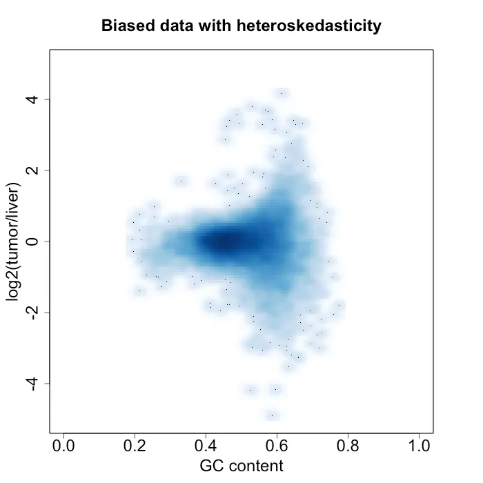
Figure 2: density plot of log2(tumor / liver) vs GC content. In this sample, the normal control sample is a liver sample.
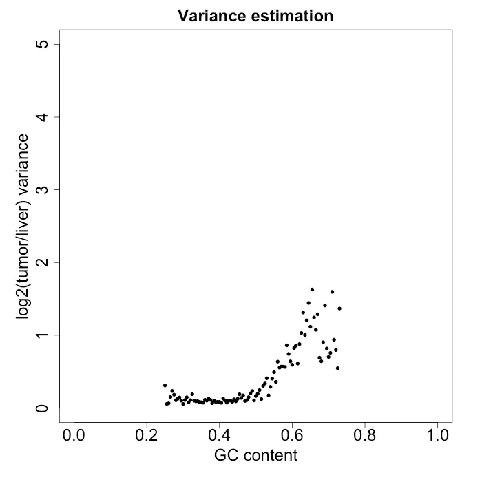
Figure 3: variance estimate in windows of GC content of 0.005. In this sample, the normal control sample is a liver sample.
DGLM method
The DGLM models the mean and dispersion simultanously (where the generalized linear model only models the mean). The variance estimates shown in Figure 3 might be amenable to some polynomial fit. So I tried two model approaches as shown below and compared the fit with RMSE and AIC:
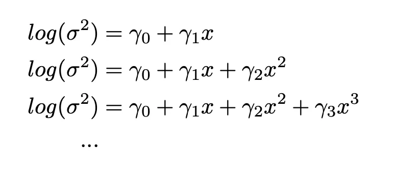
Equation 1: model approach 1 (nested approach)
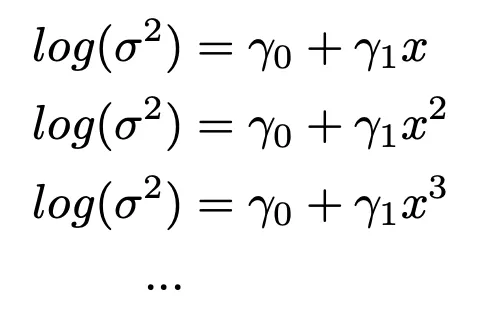
Equation 2: model approach 2 (non-nested approach)
Figures 4 and 5 show the performance of the two models while varying the parameter n. For the nested approach, n=3 seems to work best, while for the non-nested approach n=3 or n=4 seems fine. Moreover, it seems that the best nested model outperforms the best non-nested model in both AIC and RMSE. However, one issue I encountered with using DGLM is that it did not always converge with larger amounts of data and varying model complexity. I had to subsample my dataset in order to help it along.

Figure 4: AIC and RMSE of model approach 1 with varying n.
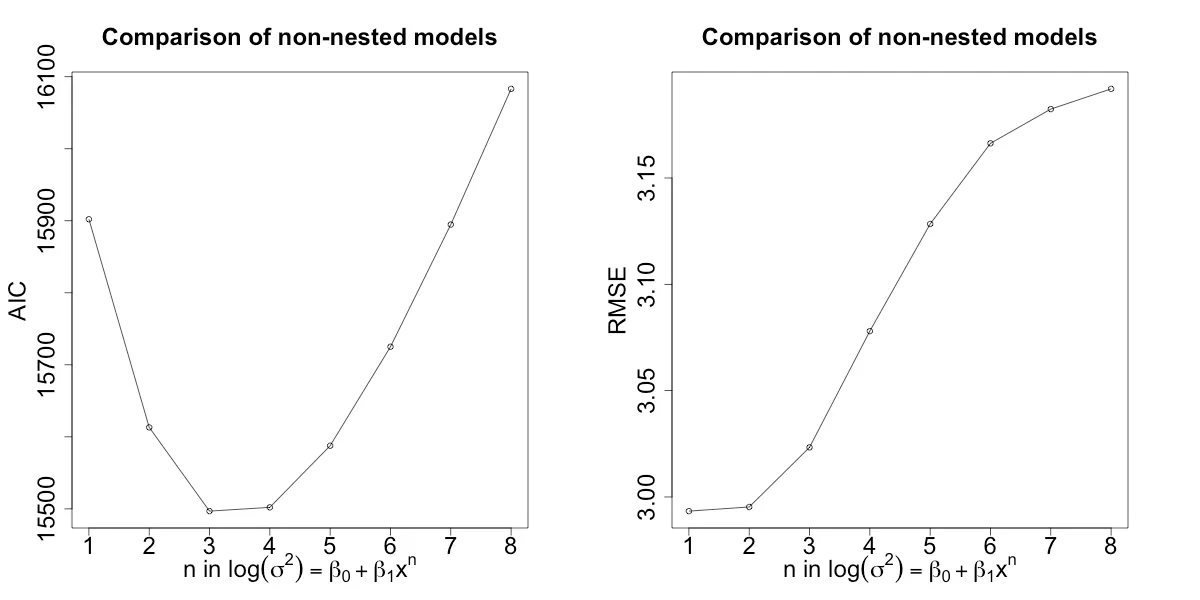
Figure 5: AIC and RMSE of model approach 1 with varying n.
LOESS method
I trained a LOESS model (10-fold cross-validtion) on the data in Figure 3 over varying varying values of the span and degree parameters. Figure 6 shows the train and test RMSE. A degree of 2 performes better over most values of span. Moreover, test error seems to be lowest for both values of degree when span is between 0.25 and 0.5. I then chose span = 0.42 and degree = 2 for my model parameters.

Figure 6: Train and test RMSE over varing degree and span parameters using 10-fold cross-validation.
Bias correction with the best models
I then took the best model from the LOESS and DGLM methods and performed the correction to my data. Figure 7 shows the variance estimates from the best model from each approach. Both seem to fit the variance pretty well. However, LOESS seems to fit the data slightly better, whereas DGLM approach shows some model bias (especially with lower GC content) likely due to using a linear equation for modeling variance. I then used each methed to correct the original data from Figure 2 using the following Equation 3, which gives the corrected data in Figure 8. Surprisingly, both approaches seem to do a pretty good job of removing the heteroskedasticity.
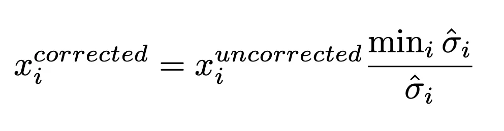
Equation 3: is the ith value, and sigma is standard deviation estimated for. Standard deviation is used because variance seems to over-correct the data and ends up not removing heteroskedasticity.
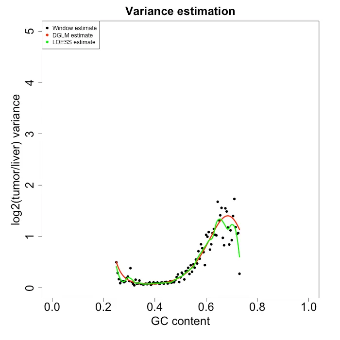
Figure 7: Variance esimate from each model approach.
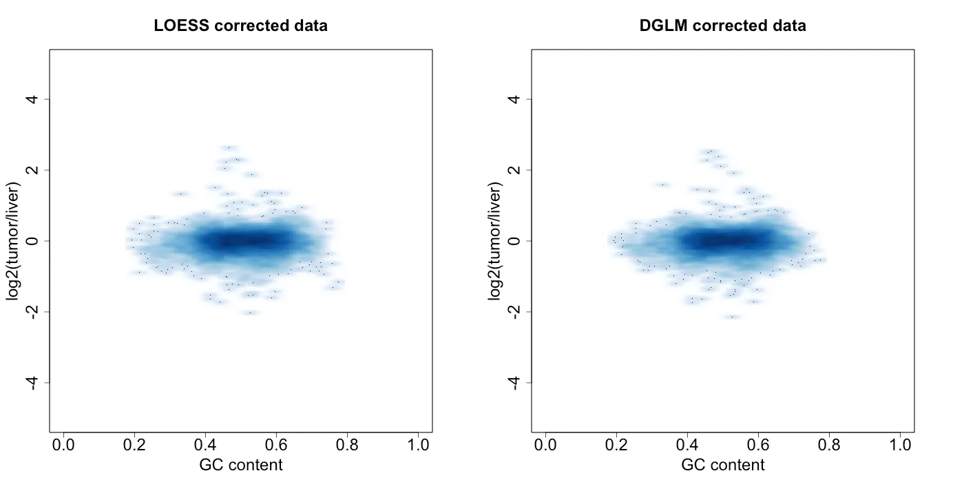
Figure 8: density plot of log2(tumor / liver) vs GC percentage
Conclusions
DGLM and LOESS both perform pretty well for removing the heteroskedasticity. LOESS is a bit more flexible in what it can model, but the downside is it can possible overfit the date. However, the test RMSE gave a pretty clear set of parameters to choose and the difference in test and train RMSE at those parameters was fairly small. DGLM on the otherhand more smoothly fits the data, which can possibly lead to some bias. Another downsite to DGLM is that it did not alway converge with larger amounts of data and varying model complexity.
Understanding the cause of the heteroskedasticity would also help decide which model to choose. It might tell us whether we expect the variance to jump around or smoothly change with GC content. But we do not know what that cause of the heteroskedasticity was…
So in the end, I would probably go with LOESS if I had to apply this approach to future data.
References
- Beroukhim R, Mermel CH, Porter D, Wei G, Raychaudhuri S, Donovan J, et al. The landscape of somatic copy-number alteration across human cancers. Nature. 2010 Feb 18;463(7283):899–905.
- Liu H, Murphy CJ, Karreth FA, Emdal KB, Yang K, White FM, et al. Identifying and Targeting Sporadic Oncogenic Genetic Aberrations in Mouse Models of Triple-Negative Breast Cancer. Cancer Discovery. 2017 Dec 4;8(3):354–69.