Code for this post.

Data exploration

This Kaggle data set is composed of 39,774 recipes from 20 cuisines (e.g. indian, spanish, etc…) Here is one example Greek recipe (JSON format):

{
    "id": 10259,
    "cuisine": "greek",
    "ingredients": [
        "romaine lettuce","black olives","grape tomatoes",
        "garlic","pepper","purple onion","seasoning",
        "garbanzo beans","feta cheese crumbles"
    ]
}

Of the 20 cuisines, the italian cuisine has the most recipes while the brazilian cuisine has the least (Figure 1).

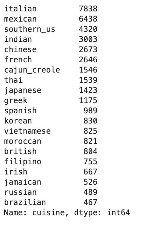
Figure 1: Count of the number recipes for each cuisine

One of the challenging aspects in this data set is that among the 6,704 ingredients there are quite a few cases where there are several names for basically the same or similar thing. Take ingredients that contain the word garlic for instance:

- Spice Islands Garlic Powder
- Spice Islands Minced Garlic
- wild garlic
- McCormick Garlic Powder
- garlic paste
- powdered garlic
- garlic salt
- etc...

A related issue is that most ingredients occur in very few recipes. While things like salt (18,048 recipes), onions (6,704 recipes), and olive oil (6,704 recipes) are the three most common ingredients, there are many, many ingredients that occur in 1 or 2 recipes (e.g. gluten-free broth, riso, cappuccino, etc…) Below I plotted a histogram of the number of recipes each ingredient occurs in (Figure 2).

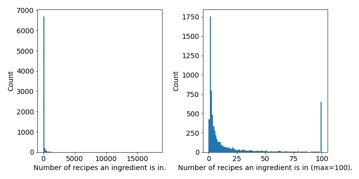
Figure 2: Both plots show a histogram of the number of recipes an ingredient occurs in, but the right figure caps it at 100.

As you’ll see, the above issues of (i) equal weighting of ingredients regardless of their abundance and (ii) redundant naming of ingredients led to less-than-ideal performance. In contrast to the t-SNE plot shown in this post’s header image, below is the same t-SNE plot using the raw dataset of 39,774 recipes and 6,704 ingredients (Figure 3). No clean group separation can be obtained even when trying various levels of perplexity. This lack of separation is likely due to all the noise from the above issues blurring the spatial structure between the cuisines.

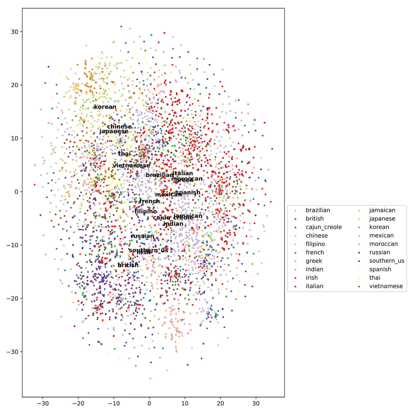
Figure 3: t-SNE plot using matrix of 1’s and 0’s for the 39,774 recipes and 6,704 ingredients. Note: as in the main header image, I am only plotting 10,000 recipes to save on computational time. The text labels are placed at the median of each cusine’s recipes.

Testing out some models

I next tried training using various models using. Admittedly, I knew beforehand that this would probably not give the best results, but it was a simple first try. The first model I thought to try is Naive Bayes:

model = MultinomialNB()
param_grid = {'alpha': [0, 0.01, 0.05,0.1,0.5,1,2,5,10]}
grid_search = GridSearchCV(model, param_grid, cv=10, n_jobs=4, scoring='accuracy')
grid_search.fit(X, y)

The alpha parameter is a smoothing parameter that helps account for variables not present during the cross validation process, which is likely to happen due to how few recipes most ingredients are in. As shown in the graph below, a very small alpha (0.05) achieved the best test accuracy of 0.7547 (Figure 4). Surprisingly, this result is pretty good in comparison to the best score on the Kaggle leaderboard is 0.83216.

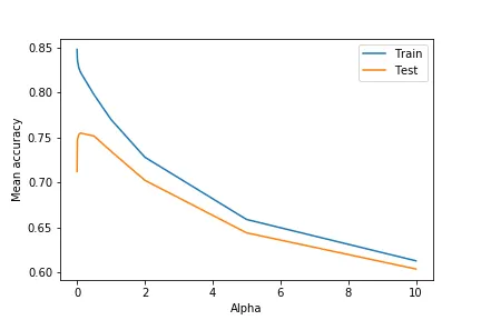
Figure 4: Test and train accuracy from 10-fold cross validation for Naive Bayes model with varying alpha.

I am not trying to be exhaustive, but I also tried a few other approaches:

• **Complement Naive Bayes (CNB): **is basically NB, but is designed to work for datasets with imbalanced class sizes, which is not so much the case I have with this data set… but I wanted to try it.
• **Regularized logistic regression (LR): **is another simple approach, but I can tweak the regularization parameter to give less weight to the less important features. I tried LR using the one-vs-one and one-vs-rest classification schemes.
• **Support vector machine (SVC): **support vector machines do well in high dimensional datasets. I tried both linear and non-linear approaches, as well as trying both one-vs-one and one-vs-rest classification schemes.

I performed 10-fold cross validation (but 5 for SVC models for performance reasons). The results mean test accuracy for the best model after grid search are shown below (Figure 5). Not surprisingly the Naive Bayes models don’t do well. LR and SVC models did best and achieved slight improvement when using the one-vs-rest classification scheme.

Figure 5: Comparison of models using max test accuracy after 10-fold cross validation (or 5 for SVC models). NB: Naive Bayes, CNB: complement Naive Bayes, LR: logistic regression, LR-OVR: logistic regression with one-vs-all scheme, LSVC: linear support vector machine, SVC: support vector machine, SVC-OVR: support vector machine with one-vs-all scheme.

Some feature engineering

Now I wanted to see how some feature engineering can improve model performance. A couple simple approaches I tried are: (1) tf-idf and (2) stemming and lemmatization.

1. tf-idf tf-idf stands for term frequency-inverse document frequency. A concept originally from text mining, it is an approach that tries to reveal how important a term is in a document compare to other documents.

2. Stemming and lemmatization This is a sort of word normalization that aims to reduce the inflectional forms of a word to its root form. E.g. “car”, “cars”, and “car’s” become “car”. Stemming and lemmatization differ in their approach to achieve that root form, but I just tried stemming for this dataset.

Applying both tf-idf and stemming (using the nltk package) reduces the number of features to 3,010 (compared to 6,704 before). I again used t-SNE to visualized the data, and this time got much better separation betwene cuisines (Figure 6).

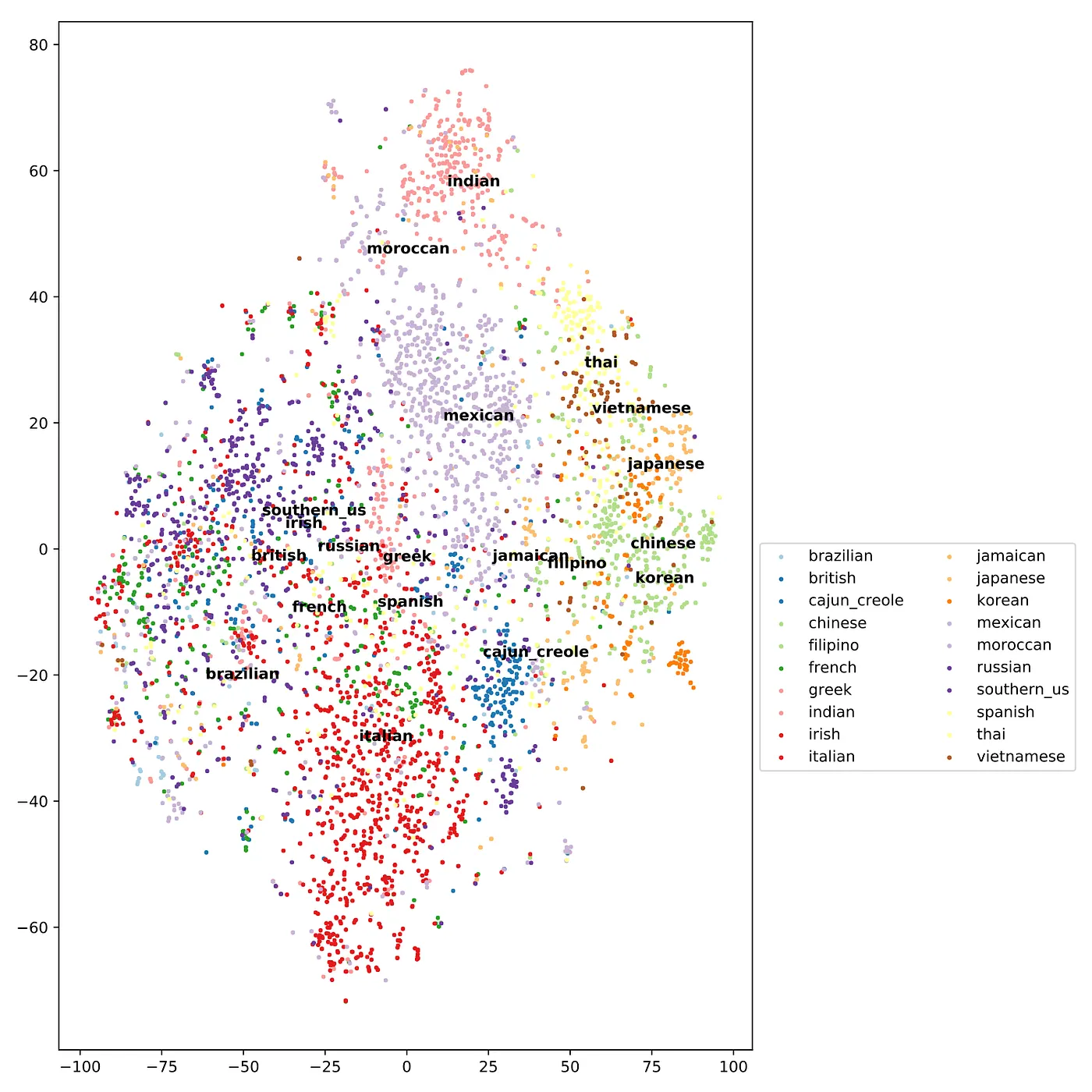
Figure 6: t-SNE plot after applying tf-idf and stemming. There are 39,774 recipes and 3,010 ingredients. Note: as in the main header image, I am only plotting 10,000 recipes to save on computational time. The text labels are placed at the median of each cuisine’s recipes.

I applied all the same classification algorithms as before (Figure 7). For most models the accuracy improved except for Naive Bayes models. The best model before was 0.7842, but after applying tf-idf and stemming it was increased to 0.816. In comparison, the best score on the Kaggle leaderboard is 0.83216.

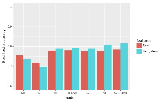
Figure 7: Comparison of models using max test accuracy after 10-fold cross validation (or 5 for SVC models). Also shows comparison of models on raw data and after transformation with tf-idf and stemming. NB: Naive Bayes, CNB: complement Naive Bayes, LR: logistic regression, LR-OVR: logistic regression with one-vs-all scheme, LSVC: linear support vector machine, SVC: support vector machine, SVC-OVR: support vector machine with one-vs-all scheme.

Conclusions

The main takeaways from this analysis are the following:

• The data consists of 39,774 recipes from 20 cuisines using 6,704 ingredients, and had two main difficulties: -The redundancy in the dataset (e.g. Spice Islands Garlic Powder, garlic powder, McCormick Garlic Powder, …)
• Most ingredients were observed in very few recipes.
• Initial attempts at dimensionality reduction for visualization were not successful, but applying some simple models achieved pretty decent performance (accuracy of 0.7547)
• Showed how feature engineering can improve accuracy (I used tf-idf and stemming) by reducing the number of features down to 3,010. This also significantly improved visualization and grouping of data via t-SNE. It also improved the accuracy of all models tried with the exception of Naive Bayes.
• Overall, support vector machine using a one-vs-all classification scheme performed the best with an accuracy of 0.816 (in comparison, 0.83216 was the best on the public Kaggle leaderboard).